Dynamic Programming 101 | Types, Examples, and Use-Cases
Say you're planning a road trip across the country. You've got a list of cities, but you can't decide on the best route. You want to complete the trip without wasting time driving back and forth. Here's how you could plan your trip in a better way:

Dynamic programming is one of the finest ways to solve a class of problems with sub-problems. Did that sound difficult to understand? Dive in to learn all about it with clear concepts and examples.
Dynamic programming (often abbreviated as DP) is a method for solving complex problems by breaking them down into simpler, smaller, more manageable parts. The results are saved, and the subproblems are optimized to obtain the best solution. The results are saved, and the subproblems are optimized to obtain the best solution. That sounds similar to so many other things, right? Well, let's start with an example.
Let's say you're planning a road trip across the country. You've got a list of cities you want to visit, but you can't decide on the best route. You want to visit all the cities without wasting too much time driving back and forth.
Here's how you could plan your trip in a better way:
Break the problem into smaller subproblems: The subproblems in this case are the routes from one city to another. You need to determine the time or distance between each pair of cities.
Solve each subproblem and store the solution: You can use a mapping app to find the shortest route (in time or distance) between each pair of cities. You then store this information for later use.
Use the solutions of the subproblems to solve the original problem: Now, using the information you've gathered and stored, you can construct the shortest possible route that visits all the cities. You start from your home city and then go to the nearest city. From there, you go to the nearest city that you haven't visited yet, and so on.
This is just a simple example of how dynamic programming works, but it gives you an idea of the process: breaking a complex problem down into simpler parts, solving each part, storing the solutions, and then combining the solutions to solve the original problem.
Table of Contents:
When to use dynamic programming
What is Dynamic Programming
Thought first by Richard Bellman in the 1950s, Dynamic Programming (DP) is a problem-solving technique used in computer science and mathematics to solve complex larger problems by breaking them down into simpler, smaller overlapping subproblems. The key idea is solving each subproblem once and storing the results to avoid redundant calculations. DP is particularly useful for problems where the solution can be expressed recursively and the same subproblem appears multiple times.
It's like tackling a giant jigsaw puzzle by piecing together smaller sections first.
Simply put, DP stores the solution to each of these smaller parts to avoid doing the same work over and over again(like you would store the shortest routes between cities in the first example). So, with dynamic programming, you're not just working harder, you're working smarter!
When to use Dynamic Programming?
So, how do you know when to use dynamic programming? There are two key hallmarks of a problem that's ripe for a DP approach:
- Overlapping Subproblems: Dynamic Programming thrives on identifying and solving overlapping subproblems. These are smaller subproblems within a larger problem that are solved independently but repeatedly. By solving and storing the results of these subproblems, we avoid redundant work and speed up the overall solution. Let’s go back to the road trip example. Imagine that the travel from City A to City B is common in several different routes. Now, instead of calculating the distance between the two cities every single time we’re mapping different routes, we can store the distance and reuse it whenever needed. This is an example of overlapping subproblems.
- Optimal Substructure: Another crucial concept is the optimal substructure property. It means that the optimal solution to a larger problem can be generated from the optimal solutions of its smaller subproblems. This property allows us to break down complex problems into simpler ones and build the solution iteratively. Let's say we've figured out the shortest route from City A to City B, and the shortest route from City B to City C. The shortest route from City A to City C via City B would be the combination of these two shortest routes. So, by knowing the optimal solutions (shortest routes) to the subproblems, we can determine the optimal solution to the original problem. That's an optimal substructure.
Practical Application: The Fibonacci Sequence
To really get a grip on dynamic programming, let's explore a classic example: The Fibonacci sequence.
It is a series of numbers in which each number is the sum of the two preceding ones, usually starting with 0 and 1.
Fibonacci Series: 0, 1, 1, 2, 3, 5, 8, 13, 21, 34…and so on.
Mathematically, we could write each term using the formula:
F(n) = F(n-1) + F(n-2),
With the base values F(0) = 0, and F(1) = 1. And we’ll follow the above relationship to calculate the other numbers. For example, F(6) is the sum of F(4) and F(5), which is equal to 8.
Let’s look at the diagram for better understanding.
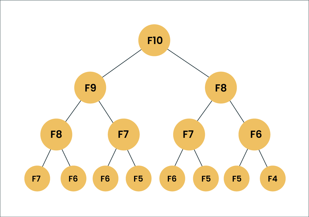
Suppose we’ve to calculate F(10). Going by the formula, F(10) should be the sum of F(8) and F(9). Similarly, F(9) would also be the sum of the subproblems F(7) and F(8). As you can see, F(8) is an overlapping subproblem here.
In the above example, if we calculate the F(8) in the right subtree, then it would result in a increased usage of resources and reduce the overall performance.
The better solution would be to store the results of the already computed subproblems in an array. First, we’ll solve F(6) and F(7) which will give us the solution to F(8) and we’ll store that solution in an array and so on. Now when we calculate F(9), we already have the solutions to F(7) and F(8) stored in an array and we can just reuse them. F(10) can be solved using the solutions of F(8) and F(9), both of which are already stored in an array.
Similarly, at each iteration we store the solutions so we don’t have to solve them again and again. This is the main attribute of dynamic programming.
If you try to compute this sequence with a straightforward recursive function, you'll end up doing a lot of unnecessary work. (Want to understand recursion from scratch?)
Here's a simple Python implementation using DP to calculate a Fibonacci sequence:
def fibonacci(n):
    # Create an array of size (n+1) to store the computed values
    dp = [0, 1] + [0] * (n - 1)

    for i in range(2, n + 1):
        # Compute the ith Fibonacci number
        dp[i] = dp[i - 1] + dp[i - 2]

    return dp[n]

print(fibonacci(10))  # Outputs: 55
Step-by-Step Approach to DP
Let's explore how to implement dynamic programming step-by-step:
- Grasp the Problem
- Find the Overlapping Subproblems
- Compute and Store Solutions
- Construct the Solution to the Main Problem
Types of Dynamic Programming
Dynamic programming is divided into two main approaches: top-down (memoization) and bottom-up (tabulation). Both of these methods help in solving complex problems more efficiently by storing and reusing solutions of overlapping subproblems, but they differ in the way they go about it.
Let's dive into these two approaches:
Top-Down DP (Memoization)
In the top-down approach, also known as memoization, we start with the original problem and break it down into subproblems. Think of it like starting at the top of a tree and working your way down to the leaves.
Here, problems are broken into smaller ones, and the answers are reused when needed. With every step, larger, more complex problems become tinier, less complicated, and, thus, faster to solve, and the results of each subproblem are stored in a data structure like a dictionary or array to avoid recalculating them. The ‘memoization’ (a key technique in DP where you store and retrieve previously computed values) process is equivalent to adding the recursion (any function that calls itself again and again) and caching steps.
Some parts can be reused for the same problem and solved when requested, making them easier to debug. However, this approach results in more memory in the call stack being occupied, which can result in a reduction in overall performance and stack overflow.
Let's revisit the Fibonacci sequence example:
def fibonacci(n, memo = {}):
    if n <= 2:
        return 1
    elif n in memo:
        return memo[n]
    else:
        memo[n] = fibonacci(n-1, memo) + fibonacci(n-2, memo)
        return memo[n]

print(fibonacci(10))  # Outputs: 55
Here, memo is a dictionary that stores the previously computed numbers. Before we compute a new Fibonacci number, we first check if it's already in memo. If it is, we just return the stored value. If it's not, we compute it, store it in memo, and then return it.
Bottom-Up DP (Tabulation)
The bottom-up approach, also known as tabulation, takes the opposite direction. This approach solves problems by breaking them up into smaller ones, solving the problem with the smallest mathematical value, and then working up to the problem with the biggest value. Solutions to its subproblems are compiled in a way that falls and loops back on itself. Users can opt to rewrite the problem by initially solving the smaller subproblems and then carrying those solutions for solving the larger subproblems.
Here, we fill up a table (hence the name "tabulation") in a manner that uses the previously filled values in the table. This way, by the time we come to the problem at hand, we already have the solutions to the subproblems we need.
Let's use the Fibonacci sequence again to illustrate the bottom-up approach:
def fibonacci(n):
    fib_table = [0, 1] + [0]*(n-1)

    for i in range(2, n+1):
        fib_table[i] = fib_table[i-1] + fib_table[i-2]

    return fib_table[n]

print(fibonacci(10))  # Outputs: 55
In this case, fib_table is an array that stores the Fibonacci numbers in order. We start by filling in the first two numbers (0 and 1), and then we iteratively compute the rest from these initial numbers.
In contrast to the top-down approach, the bottom-up approach relies on eliminating recursion functions. There is no stack overflow, and memory space is saved with reduced timing complexity, making it more efficient and preferred when the order of solving subproblems is not critical.
Which approach to choose?
Both top-down and bottom-up dynamic programming can be useful, and your choice depends on the problem at hand and the specific requirements of your program.
The top-down approach might be easier to understand because it follows the natural logic of the problem, but it can involve a lot of recursion and may have a larger memory footprint due to the call stack.
On the other hand, the bottom-up approach can be more efficient because it avoids recursion and uses a loop instead, but it might require a better understanding of the problem to build the solution iteratively.
What are the signs of DP suitability?
Identifying whether a problem is suitable for solving with dynamic programming (DP) involves recognizing certain signs or characteristics that suggest DP could be an effective approach. Here are some common signs that indicate a problem might be a good fit for dynamic programming:
- Overlapping Subproblems: A problem that can be broken down into smaller subproblems that are solved independently, and the same subproblems encountered multiple times strongly indicates DP suitability.
- Optimal Substructure: Problems that exhibit optimal substructure can often be solved using DP. This means that the optimal solution for a larger problem can be constructed from the optimal solutions of its smaller subproblems.
- Recursive Nature: Problems that can be naturally expressed using recursion are often well-suited for DP.
- Memoization Opportunities: If you notice that you can improve a recursive algorithm by memoizing (caching) intermediate results, DP might be a good fit.
- Sequential Dependencies: Problems where the solution depends on the results of previous steps or stages are often candidates for DP. DP is particularly useful when solving problems involving sequences, such as strings, arrays, or graphs.
- Optimization or Counting: DP is often applied to optimization problems (maximizing or minimizing a value) or counting problems (finding the number of possible solutions).
- Recursive Backtracking Inefficiency: If you encounter a recursive backtracking algorithm that is slow due to repeated calculations, this is a clear indication that DP might be a better approach.
- Subproblem Independence: Some problems have subproblems that are entirely independent of each other. In such cases, DP can be applied to solve each subproblem in parallel or any order, making it an efficient choice.
- Limited Set of Choices: Problems where the number of choices at each step is limited and doesn't grow exponentially can often be tackled with DP. DP can explore all possible choices without leading to an impractical number of computations.
Final Thoughts
Dynamic programming is a little like magic: It turns a daunting problem into a series of manageable tasks, making the impossible possible. But unlike a magic trick, the method behind dynamic programming is logical and grounded in sound reasoning.
Sure, getting the hang of it might take some time. You'll need to practice spotting overlapping subproblems and constructing optimal solutions. But once you've mastered these skills, you'll be able to tackle a wide range of problems with newfound efficiency.
Dynamic programming is a useful but advanced skill to learn if one is a programmer or DevOps engineer, particularly if you specialize in Python. It makes complex algorithmic problems easy to digest and its versatility makes it a must-have in the repertoire of every DevOps learning kit. Remember, the journey of a thousand miles begins with a single step – or in our case, a single subproblem.
Cheers and Happy Coding!
FAQs on Dynamic Programming
When should I use Dynamic Programming?
Use Dynamic Programming when you encounter problems with overlapping subproblems and optimal substructure. Common applications include algorithms for optimization, like finding the shortest path, maximizing profit, or minimizing cost.
Are there different types of Dynamic Programming?
Yes, Dynamic Programming can be categorized into two main types: Memoization (Top-down) and Tabulation (Bottom-up). The choice between them depends on the specific problem and your coding preferences.
Learn more:
The Art of Debugging: Mastering the Bug Hunt, One Error at a Time
Introduction to Object-Oriented Programming
How Software is Developed? A Step-By-Step Guide