
Time complexity and Big O notation for beginners
Big O notation for beginners: the classes from O(1) to O(2^n) with examples, how to read code, amortised cost, space complexity and the limits of Big O.

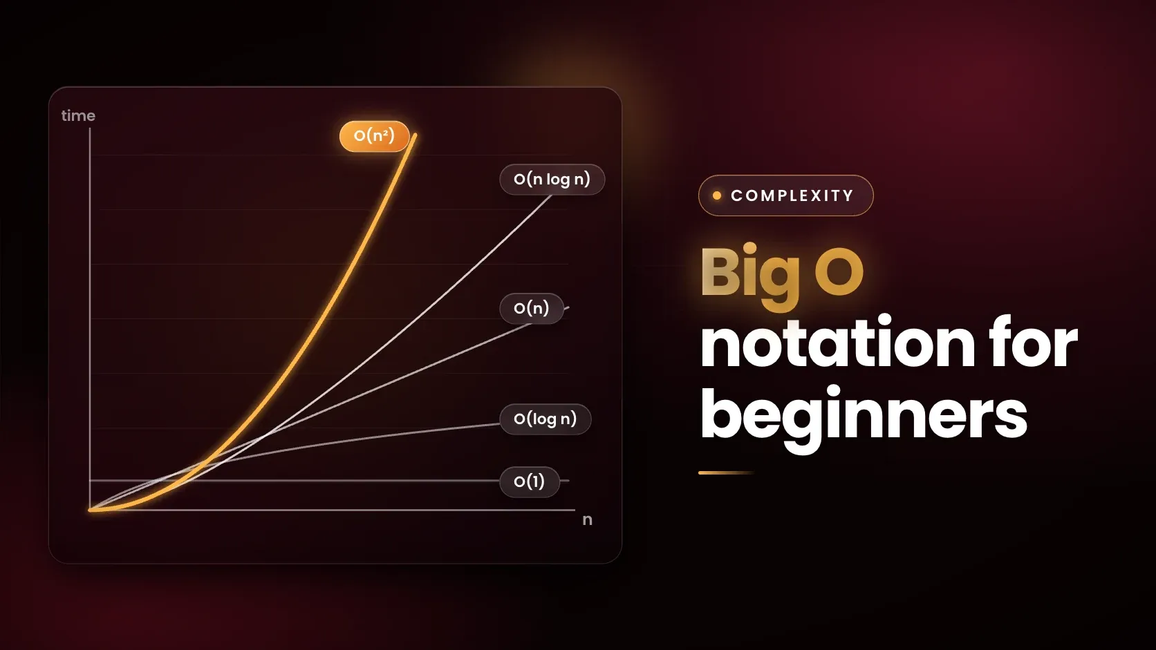
Big O notation describes how an algorithm's running time or memory grows as the input size n grows, ignoring constant factors. O(1) is constant, O(log n) logarithmic, O(n) linear, O(n log n) linearithmic, O(n^2) quadratic and O(2^n) exponential. NIST defines f(n) = O(g(n)) as f staying below a constant multiple of g once n is large enough.
What does Big O notation measure?
Big O measures growth, not seconds. NIST's Dictionary of Algorithms and Data Structures calls it a theoretical measure of the execution of an algorithm, usually the time or memory needed, given the problem size n. The formal definition says f(n) = O(g(n)) when positive constants c and k exist such that f(n) is at most c times g(n) for every n from k onwards.
Two rules follow. Constants and lower-order terms are dropped, because NIST's own example shows n^2 + 3n + 4 is O(n^2). And Big O is an upper bound. Princeton's lecture slides describe Big Oh as "Theta(N^2) and smaller", used to develop upper bounds, while Big Theta is the tight bound used to classify an algorithm. Writing O(n^2) for a linear algorithm is technically true and unhelpful, which is why NIST warns that Big O is often misused to mean "equal to".
Worst case and Big O are separate ideas. Worst case is about which input is hardest. Big O is about how a cost function grows. An algorithm can have a Big O bound for its best case, its average case and its worst case.
What are the common time complexity classes?
Seven classes cover most everyday code. The Competitive Programmer's Handbook and Princeton's Algorithms course list the same set, and the table pairs each class with its usual code shape and what happens to the running time when the input size doubles.
| Class | Name | Typical code shape | Example | Input doubles |
|---|---|---|---|---|
| O(1) | Constant | A single statement | Read a[0] | No change |
| O(log n) | Logarithmic | Halve the input each step | Binary search | One extra step |
| O(n) | Linear | One loop | Find the maximum | About 2 times |
| O(n log n) | Linearithmic | Divide and conquer | Merge sort | A little over 2 times |
| O(n^2) | Quadratic | Two nested loops | Compare all pairs | 4 times |
| O(n^3) | Cubic | Three nested loops | Check all triples | 8 times |
| O(2^n) | Exponential | Try every subset | Subset search | Each extra item doubles it |
Princeton's slides state that the functions 1, log N, N, N log N, N^2, N^3 and 2^N suffice to describe the order of growth of most common algorithms. The Handbook adds a factorial class, for code that tries every permutation of the input.
What is the difference between O(n) and O(log n)?
An O(n) algorithm does work proportional to the input size, while an O(log n) algorithm does work proportional to the number of times the input can be halved. Searching 1,000,000 sorted items one by one can take 1,000,000 steps. Halving the range each time, as binary search does, takes at most 20.
The next code block counts steps for three shapes at three sizes. The linear pass takes n steps, the double loop takes n squared, and halving takes about log2 n.
def linear(a):               # O(n): one pass
    steps = 0
    for x in a:
        steps += 1
    return steps

def quadratic(a):            # O(n^2): every pair
    steps = 0
    for x in a:
        for y in a:
            steps += 1
    return steps

def logarithmic(n):          # O(log n): halve until 1
    steps = 0
    while n > 1:
        n //= 2
        steps += 1
    return steps

print("n      linear  quadratic  halving")
for n in (10, 100, 1000):
    a = list(range(n))
    print(f"{n:<6} {linear(a):<7} {quadratic(a):<10} {logarithmic(n)}")
n linear quadratic halving
10 10 100 3
100 100 10000 6
1000 1000 1000000 9Growth rates separate quickly. The table gives exact values for small n, which is where the exponential class first stands out.
| n | log2 n | n | n log2 n | n^2 | 2^n |
|---|---|---|---|---|---|
| 10 | 3.32 | 10 | 33.2 | 100 | 1,024 |
| 20 | 4.32 | 20 | 86.4 | 400 | 1,048,576 |
| 30 | 4.91 | 30 | 147.2 | 900 | 1,073,741,824 |
At n = 1,000 the same formulas give about 9,966 for n log2 n against 1,000,000 for n^2.
How do you calculate the time complexity of code?
Count how many times the dominant statement runs as a function of n, then keep the fastest-growing term. The Competitive Programmer's Handbook gives the working rules:
- Statements run one after another add their costs, so an O(n) loop followed by an O(n^2) loop is O(n^2).
- Nested loops multiply, so a loop of n inside a loop of n is O(n^2), and loops over two inputs of sizes n and m give O(nm).
- A loop that halves its counter, such as
while n > 1: n //= 2, runs about log2 n times. - For recursion, multiply the number of calls by the cost of one call.
The recursion rule explains the most famous slow function. A function that calls itself once with n - 1 makes n calls and is O(n). A function that calls itself twice with n - 1 makes 1 + 2 + 4 + ... + 2^(n-1) calls, which the Handbook totals as 2^n - 1, so it is O(2^n). Naive recursive Fibonacci has this shape. Remembering results, called memoisation, collapses it to O(n).
calls = 0
def fib(n):                  # O(2^n): two recursive calls per call
    global calls
    calls += 1
    return n if n < 2 else fib(n - 1) + fib(n - 2)

memo, memo_calls = {}, 0
def fib_memo(n):             # O(n): each value computed once
    global memo_calls
    memo_calls += 1
    if n not in memo:
        memo[n] = n if n < 2 else fib_memo(n - 1) + fib_memo(n - 2)
    return memo[n]

for n in (10, 20, 30):
    calls, memo, memo_calls = 0, {}, 0
    fib(n); fib_memo(n)
    print(n, calls, memo_calls)
10 177 19
20 21891 39
30 2692537 59For n = 30 the naive version makes 2,692,537 calls and the memoised version 59. A tree traversal, by contrast, visits each node once, so it is O(n), as shown in binary tree traversal.
What is amortised cost?
Amortised cost is the average cost per operation over a whole sequence of operations, even when single operations are sometimes expensive. Princeton's Algorithms text states that in a resizing-array stack or queue, any sequence of N operations starting from empty takes time proportional to N in the worst case, which is amortised constant time per operation.
Python's list.append is the standard example. The Python documentation lists append as O(1) amortized and notes that an individual call may occasionally be O(n) when the storage is resized. The language FAQ explains that CPython lists are variable-length arrays and that extra space is allocated when the array must grow, so the next few appends need no resize. The sample below builds a doubling array by hand and counts element copies.
class DynamicArray:
    def __init__(self):
        self.capacity, self.size, self.copies = 1, 0, 0
        self.data = [None] * self.capacity

    def append(self, x):
        if self.size == self.capacity:           # full: double and copy everything
            self.capacity *= 2
            new = [None] * self.capacity
            for i in range(self.size):
                new[i] = self.data[i]
                self.copies += 1
            self.data = new
        self.data[self.size] = x
        self.size += 1

arr = DynamicArray()
for i in range(1000):
    arr.append(i)
print(arr.size, arr.copies, arr.copies / arr.size)
1000 1023 1.023A thousand appends cost 1,023 copies in total, about one per append. Single resizes are expensive, yet the average stays constant.
What is space complexity?
Space complexity applies the same notation to memory. NIST's definition of Big O covers time or memory, so an algorithm can be described by both. Merge sort, for instance, uses extra space proportional to N, while insertion sort works in place.
Time and space often trade against each other. The sample below checks 1,000 distinct numbers for duplicates. Nested loops use no extra memory but make 499,500 comparisons. A set remembers what it has seen, uses O(n) extra space, and needs only 1,000 steps.
def has_duplicate_pairs(a):          # time O(n^2), extra space O(1)
    steps = 0
    for i in range(len(a)):
        for j in range(i + 1, len(a)):
            steps += 1
            if a[i] == a[j]:
                return True, steps
    return False, steps

def has_duplicate_set(a):            # time O(n) on average, extra space O(n)
    seen, steps = set(), 0
    for x in a:
        steps += 1
        if x in seen:
            return True, steps
        seen.add(x)
    return False, steps

a = list(range(1000))                # no duplicates: worst case for both
print(has_duplicate_pairs(a))
print(has_duplicate_set(a))
(False, 499500)
(False, 1000)The set version is O(n) only on average. The Python documentation says set and dict operations are O(1) on average and can degrade to O(n) when every key hashes to the same value.
What are the limits of Big O in practice?
Big O ignores constants, and constants matter for small inputs. The Competitive Programmer's Handbook points out that an O(n) algorithm may perform n/2 or 5n operations. Princeton's slides list "interpreting big-Oh as an approximate model" as a common mistake, because Big O is a bound and not a prediction of running time.
Growth rate still wins as inputs get large. NIST cites a classic comparison: for 1,000,000 numbers, quicksort takes about 20,000,000 steps on average while bubble sort takes about 1,000,000,000,000, enough for a small computer running quicksort to beat a supercomputer running bubble sort. The Handbook's rule of thumb makes the same point in reverse: with a one-second limit and hundreds of millions of operations per second, O(n^2) is acceptable up to about n = 5,000, while inputs up to 1,000,000 need O(n log n) or O(n).
Other limits are worth remembering. Big O also treats every basic operation as equal in cost, although the V8 team notes that in JavaScript a comparison is usually far more expensive than a memory access, because it often calls user code. The best, average and worst cases of one algorithm can differ, as with quicksort at O(n log n) on average and O(n^2) at worst, which sorting algorithms explained works through.
An operation that looks cheap may also hide a loop: x in some_list is O(n) in Python, while x in some_set is O(1) on average, per the Python documentation. For the wider picture of how these ideas fit together, see Demystifying Data Structures and Algorithms.
Where does complexity thinking fit in data science study?
Complexity thinking decides which tool to reach for. Choosing a set over a list for membership tests, or sorting once and then using binary search instead of repeated scans, is a Big O decision. Certification in Data Science and Artificial Intelligence is an online programme from E&ICT Academy, IIT Roorkee, run with Masai as the implementation partner, with live online sessions and an optional campus immersion at IIT Roorkee, covering Python, data analysis, SQL, statistics, machine learning and generative AI.
Its modules include Programming & Data Foundations, Data Analysis with NumPy & Pandas, and SQL, Visualization & Data Storytelling. Details are on the Certification in Data Science and Artificial Intelligence page.
Frequently asked questions
What is Big O notation?
Big O notation is a way to describe how an algorithm's running time or memory use grows with input size, keeping only the fastest-growing term and dropping constants. Formally, f(n) = O(g(n)) means f is at most a fixed multiple of g for all large enough n. It gives an upper bound.
What is the difference between O(n) and O(log n)?
O(n) work grows in step with the input, so doubling the input doubles the work. O(log n) work grows by one step when the input doubles, because the input is halved each time. Searching 1,000,000 sorted items takes at most 20 steps with binary search, against up to 1,000,000 for a scan.
How do you calculate the time complexity of a program?
Count how often the busiest statement runs as a function of n. Add costs of loops that run one after another, multiply costs of nested loops, treat a loop that halves its counter as log n, and multiply calls by per-call cost for recursion. Then keep only the fastest-growing term.
What is the difference between Big O and Big Theta?
Big O is an upper bound, so an algorithm that is linear is also O(n^2). Big Theta is a tight bound, meaning the growth is within constant multiples of the function from above and below. NIST notes that Big O is often misused to mean "equal to", which is what Theta expresses.
What is amortised time complexity?
Amortised time complexity is the average cost per operation across a sequence of operations, even if some single operations are costly. Python's list append is O(1) amortized because occasional resizes are spread over many cheap appends. A thousand appends to a doubling array need 1,023 element copies in total.
Is O(1) always faster than O(n)?
No. Big O hides constant factors, so an O(1) operation with a large constant can be slower than an O(n) one on small inputs. Big O describes how cost grows as n increases, not the time of any single call, so measure when the difference matters.
Next step
Practise by writing the step-counting code for a few functions of your own and predicting the class before running it. If data analysis in Python is the next skill to build, look at the Certification in Data Science and Artificial Intelligence programme from E&ICT Academy, IIT Roorkee. A good follow-up is the heap data structure and priority queue, where insert and extract cost O(log n).