
Tree Data Structure: Types, Operations, Applications
A tree is a hierarchy of nodes joined by edges. Learn the terms, the types (binary tree, binary search tree, AVL, B-tree), the four traversals, insert, search and delete with code, time complexity and five classic interview problems.

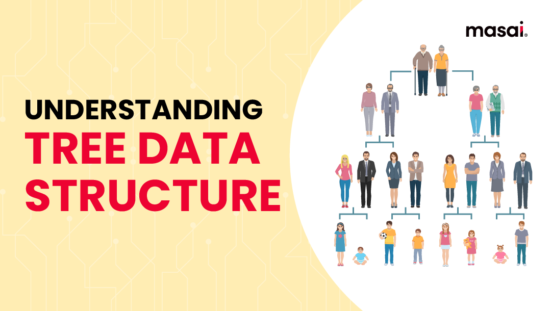
Have you made a family tree in one of those school assignments when you were a kid?
Even if you haven't, you must have seen one.
It basically starts from a root point (grandparents or maybe even great grandparents) and then spreads across multiple generations in a hierarchical order.
If you still can't picture it, just imagine an inverted tree (literally, a tree). It originates from the root and then several branches come out at different heights.
That's what a tree data structure looks like.
We've learned the linear data structures like arrays, stacks, queues, and linked lists in our previous articles. (If you haven't, please refer to this list)
What is a tree data structure?
Now, we're going to learn about a non-linear data structure - Tree.
A tree is a hierarchical data structure that contains a collection of nodes connected via edges so that each node has a value and a list of pointers to other nodes. (Similar to how parents have the reference to their children in a family tree)
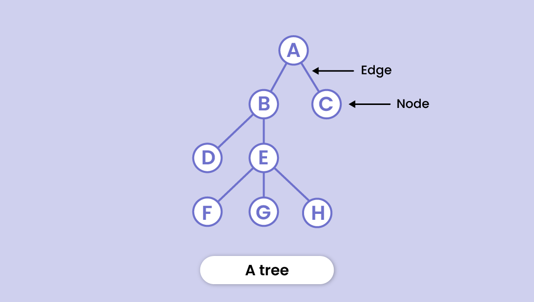
Following are the key points of a tree data structure:
- Trees are specialized to represent a hierarchy of data
- Trees can contain any type of data be it strings or numbers
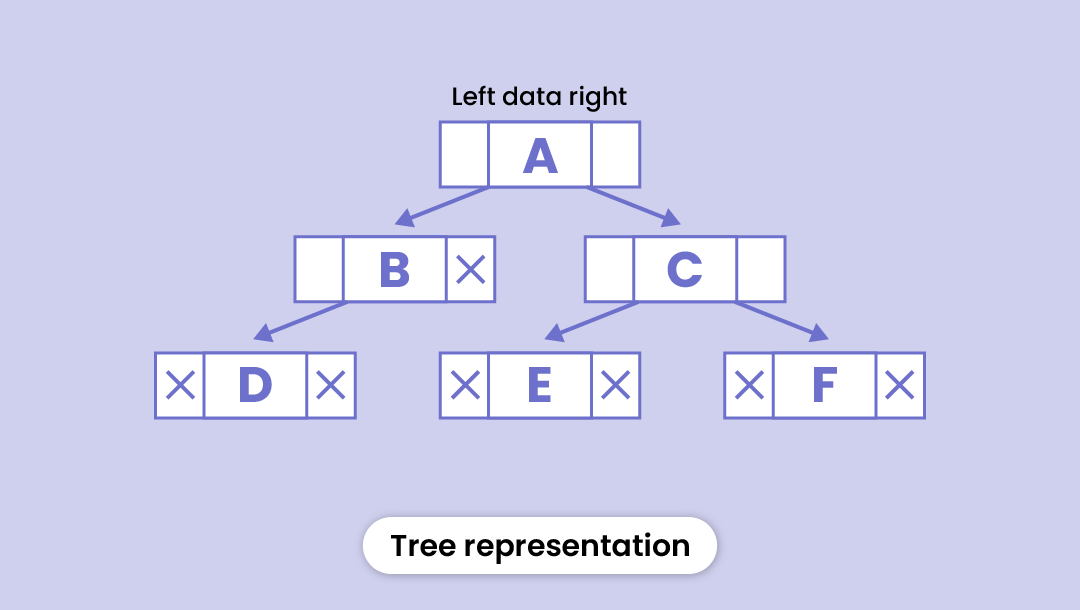
Here’s the logical representation of a tree:
A tree is a special kind of graph: it is connected and has no cycles, so there is exactly one path between any two nodes. If your data can contain cycles, such as a road map, you need a general graph instead.
Basic terms of a tree data structure
Root node
The topmost node in the tree hierarchy is known as the root node. In other words, it's the origin point of the tree that doesn't have any parent node.
Child node
A node that sits directly below another node, joined to it by an edge, is a child of that node.
Parent node
A node that has a child (a sub-node directly below it) is called the parent of that child.
Siblings
Just like a family tree, nodes having the same parent node are called siblings.
Leaf node
A leaf node is a node with no child nodes. Leaf nodes are also called external nodes. The "end" of a tree branch is normally where the leaf nodes are located.
Internal node
A node having at least one child node is known as an internal node. Internal nodes in a tree structure are often located "between" other nodes.
Ancestor Node
Any node on the path from the root down to the current node, other than the current node itself, is an ancestor. You may think of ancestor nodes as "parents, grandparents, etc."
Descendant
A descendant is any child, grandchild, great-grandchild, etc. of the current node. Any node in the tree structure that is "below" the current node is referred to as a descendent.
Edges
The link between any two nodes is called an edge.
Height
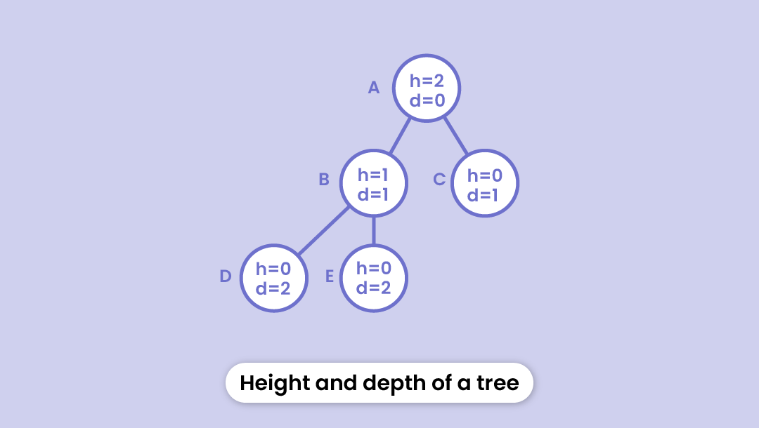
The height of a node is the number of edges on the longest path from that node down to a leaf.
In the figure below - the height of node B will be the number of edges from B to the external node i.e. D. Thus h = 1.
Depth
The depth of a node is the number of edges it takes from the root node to that particular node.
In the figure below - the depth of node D will be the number of edges from A to D. Thus d = 2.
Degree
The total number of branches coming out of a node is considered to be the degree of that node.
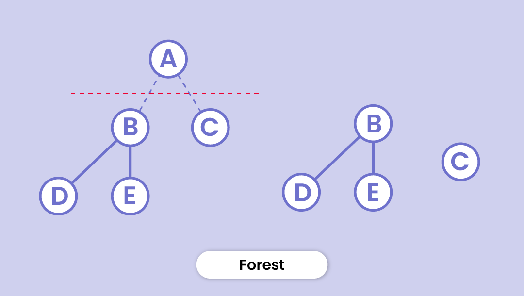
Forest
It's not hard to guess, is it? A collection of disconnected trees is called a forest. If you cut the root of a tree, the disjoint trees hence formed make up a forest. (As shown in the figure)
The characteristics of tree data structures
A tree, which replicates a hierarchical tree structure with a collection of connected nodes, is a common data structure in computer science. The following characteristics of a tree data structure:
- Number of edges
- Recursive data structure
- Height of node x
- Depth of node x
Continue reading to understand more about each of these tree data structure's characteristics in greater depth.
Number of edges: A tree's edge count is always one less than its node count. The reason: every node except the root has exactly one edge to its parent, so n nodes have n - 1 edges.
Recursive data structure: Every child node is the root of a smaller tree (a subtree), so a tree is built from smaller trees. That is why most tree algorithms are written recursively. A tree whose nodes have at most n children is called an n-ary tree.
Height of node x: The distance along the longest route leading from a node to any leaf node is used to measure a node's height. In other words, it is the number of edges on the longest path from that node down to a leaf.
Depth of node x: A node's depth is the distance along the path from the root to that node. In other words, it only refers to how many edges there are on the route leading from the root to that specific node.
Types of Trees
Binary Tree
In this data structure, each parent node can contain a maximum of two children nodes. (The left and the right child)
Each node in a binary tree contains the following three parts:
- Data
- Pointer to the left child
- Pointer to the right child
In the tree representation above, node A has two children, B on the left and C on the right. Node B has only a left child (D), so its right pointer is null. Node C has two children, E and F. Nodes D, E and F are leaf nodes, so both of their pointers are null.
There are five major types of binary trees:
Full Binary Tree - Every parent node has either two or no children.
Perfect Binary Tree - Every parent node has exactly two child nodes and all the external nodes (leaf nodes) are at the same level.
Complete Binary Tree - Every level is completely filled except possibly the last, and the last level is filled from the left.
Degenerate Tree - The tree in which the parent nodes have a single child, either left or right is called a degenerate tree.
Balanced Binary Tree - A binary tree in which, for every node, the heights of the left and right subtrees differ by at most 1.
In code, a binary tree node holds a value and two pointers. The snippets in the rest of this post build on this class:
class Node:
    def __init__(self, value):
        self.value = value
        self.left = None       # pointer to the left child (None if there is none)
        self.right = None      # pointer to the right child
Binary Search Tree
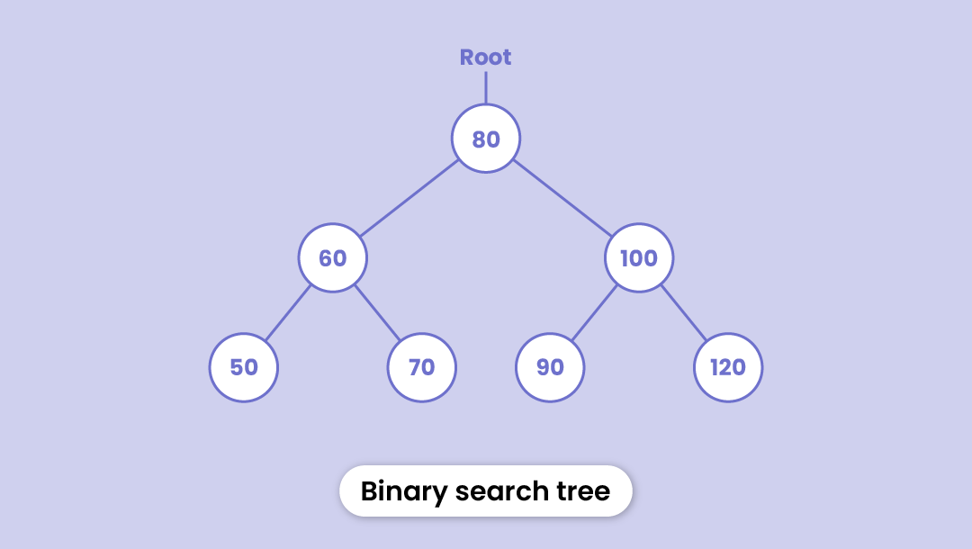
We've already learned about the binary tree.
A binary tree that maintains some order to arrange the nodes is called a binary search tree.
It is similar to a binary tree in the sense that each node can have at most two children; however, there are a few specifications:
- Each node of the left subtree has a smaller value than the root node
- Each node of the right subtree is larger than the root node
- This arrangement follows throughout the tree i.e. both subtrees of all the nodes have the same properties
The search operation is much easier in a binary search tree. If the required value is smaller than the root, we only need to search the left subtree. If it is larger, it cannot be in the left subtree, so we only search the right subtree. Each step discards a whole subtree, so a search costs O(h), where h is the height of the tree. The code is in the Searching section below.
One more useful property: an inorder traversal of a binary search tree visits the keys in sorted order.
AVL Tree
To understand AVL Tree, we first need to understand the term - Balance Factor.
The balance factor of a node is the difference between the height of the left subtree and the height of the right subtree of that particular node.
It can also be defined as a height-balanced binary search tree.
For a tree to be height balanced, the balance factor of each node must be between -1 to 1 (-1, 0, or 1).
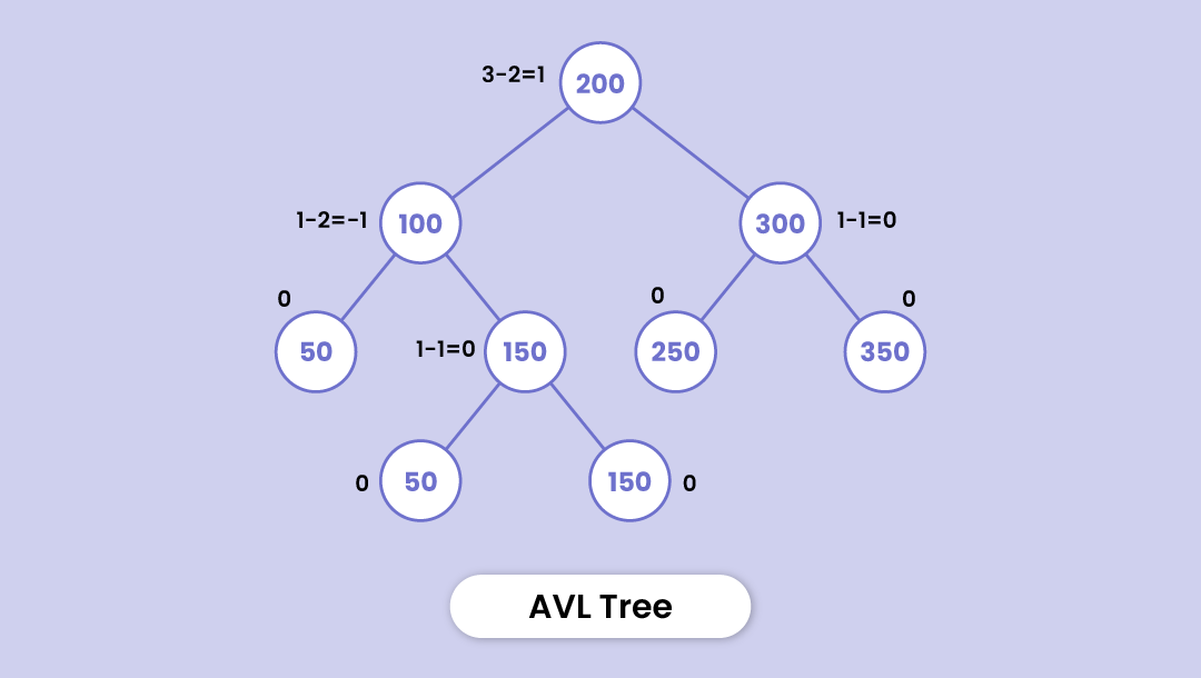
Let's understand through this example -
Here, node 200 has a balance factor of 1. How?
(Height of left child node 100 - the height of node 300)
Similarly, node 100 has a balance factor of -1; as the difference in the heights of its left subtree and the right subtree is -1.
AVL Tree allows the same search operation as a binary search tree as it follows the same properties. (Left subtree < root < right subtree )
An AVL tree rebalances itself after every insertion and deletion, so its height stays O(log n) and search, insertion and deletion take O(log n) even in the worst case. (Some books define the balance factor as right height minus left height. The allowed values, -1, 0 and 1, are the same.)
B-Tree
It's a specialized self-balancing tree in which each node can have more than one key and more than two child nodes. It's also called a height-balanced m-way tree.
With its capacity to store multiple keys, a B-tree takes much lesser time to access physical storage media like a hard disk.
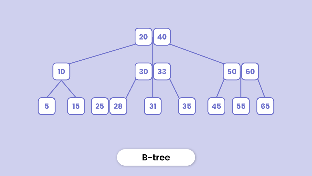
Since other tree types like binary search tree, AVL Tree, etc. can only contain one key in one node, storing a large number of keys increases their height by a stretch and the access time increases. B-tree solves this problem.
Here are a few properties of a B-tree:
- Each node in a B-Tree of 'm' order contains a maximum of 'm' children. Order in a B-tree represents the maximum number of children possible.
- The root must have at least 2 children, unless it is a leaf
- All leaf nodes are at the same level (they have the same depth)
- If the tree is of x order, each internal node can contain at most x-1 keys with a pointer to every child.
Traversal in a tree data structure
In linear data structures like arrays, stacks, etc. there's only one way to traverse the data. But, a hierarchical data structure like a tree can have different ways of traversal.
In order to traverse a tree, we need to read all the nodes in the left subtree, the root node, and all the nodes in the right subtree.
There are three depth-first ways of traversal depending on the order we want to follow, plus level-order traversal, which goes breadth-first:
Inorder traversal
- It starts with visiting all the nodes in the left subtree
- Then visits the root node
- And finally, all the nodes in the right subtree are visited
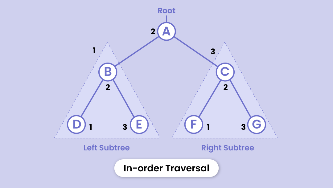
The order will be: D - B - E - A - F - C - G
Preorder traversal
- First, the root node is visited
- Then all the nodes in the left subtree
- And finally visits all the nodes in the right subtree
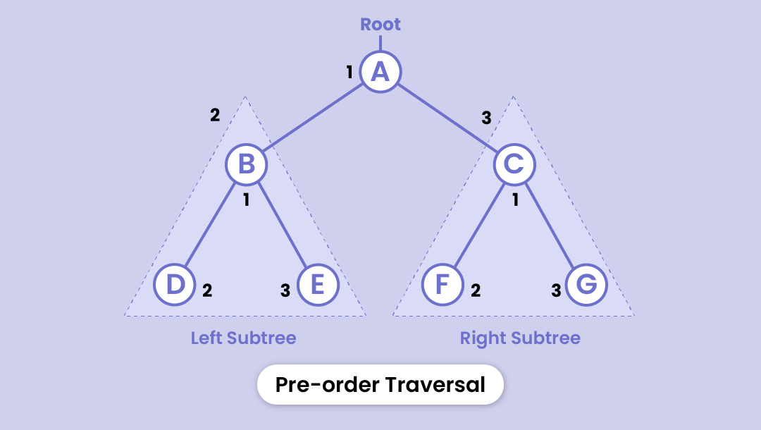
The order will be: A - B - D - E - C - F - G
Post-order traversal
- Starts with the nodes in the left subtree
- Visits the nodes in the right subtree
- And then visits the root node
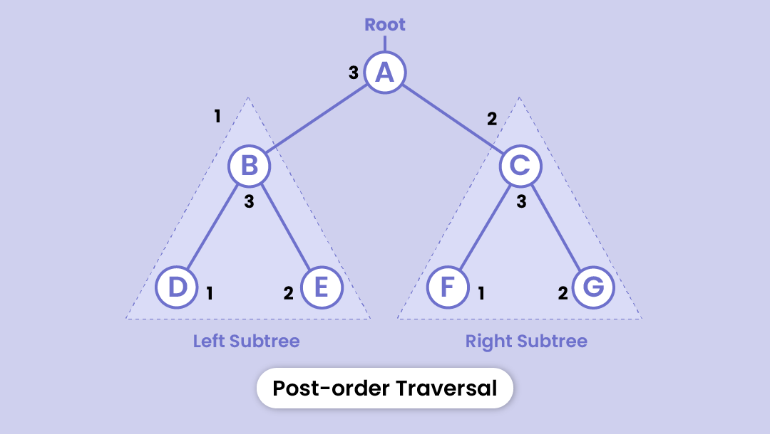
Here, the order will go as D - E - B - F - G - C - A
Level-order traversal
Level-order traversal visits the nodes level by level, left to right, using a queue. For the same tree, the order is A - B - C - D - E - F - G.
Here are all four traversals in Python. The three depth-first ones are naturally recursive (see how recursion works), and every traversal visits each node once, so it takes O(n) time:
from collections import deque

# the tree from the traversal diagrams: A has B and C, B has D and E, C has F and G
root = Node("A")
root.left, root.right = Node("B"), Node("C")
root.left.left, root.left.right = Node("D"), Node("E")
root.right.left, root.right.right = Node("F"), Node("G")

def preorder(node, out):                 # root, left, right
    if node:
        out.append(node.value)
        preorder(node.left, out)
        preorder(node.right, out)
    return out

def inorder(node, out):                  # left, root, right
    if node:
        inorder(node.left, out)
        out.append(node.value)
        inorder(node.right, out)
    return out

def postorder(node, out):                # left, right, root
    if node:
        postorder(node.left, out)
        postorder(node.right, out)
        out.append(node.value)
    return out

def level_order(node):                   # level by level, using a queue
    order, queue = [], deque([node])
    while queue:
        current = queue.popleft()
        if current:
            order.append(current.value)
            queue.append(current.left)
            queue.append(current.right)
    return order

print(preorder(root, []))     # ['A', 'B', 'D', 'E', 'C', 'F', 'G']
print(inorder(root, []))      # ['D', 'B', 'E', 'A', 'F', 'C', 'G']
print(postorder(root, []))    # ['D', 'E', 'B', 'F', 'G', 'C', 'A']
print(level_order(root))      # ['A', 'B', 'C', 'D', 'E', 'F', 'G']
Basic operations of a tree
Here are a few basic operations you can perform on a tree: insertion, searching and deletion, plus the traversals above. The code below mostly uses a binary search tree, the most common case, and builds on the Node class from the binary tree section.
Insertion
Where a new node goes depends on the kind of tree:
- General binary tree: put the new node in the first vacant position you find while walking the tree level by level. This keeps the tree compact.
- Binary search tree: the ordering decides. Go left if the new value is smaller and right if it is larger, and attach the node where you reach an empty spot.
First vacant position in a general binary tree:
def insert_first_vacant(root, value):    # general binary tree: fill the first gap, level by level
    new = Node(value)
    if root is None:
        return new
    queue = deque([root])
    while queue:
        current = queue.popleft()
        if current.left is None:
            current.left = new
            return root
        if current.right is None:
            current.right = new
            return root
        queue.append(current.left)
        queue.append(current.right)

tree = None
for v in [1, 2, 3, 4, 5]:
    tree = insert_first_vacant(tree, v)
print(level_order(tree))      # [1, 2, 3, 4, 5]
Insertion in a binary search tree. Inserting the keys below gives the tree that appears in the deletion picture, and an inorder walk returns them sorted:
def insert(root, value):                 # binary search tree
    if root is None:                     # empty spot found: the new node goes here
        return Node(value)
    if value < root.value:
        root.left = insert(root.left, value)
    elif value > root.value:
        root.right = insert(root.right, value)
    return root                          # equal keys are ignored: BST keys are unique

bst = None
for v in [100, 50, 150, 12, 60, 120, 104, 140]:
    bst = insert(bst, v)
print(inorder(bst, []))       # [12, 50, 60, 100, 104, 120, 140, 150]  (sorted)
Searching
In a binary search tree each comparison discards one subtree, so the search follows a single path from the root. In a general binary tree there is no ordering, so you check the current node and then both subtrees, which takes O(n) time.
def search(root, value):
    if root is None or root.value == value:
        return root                      # found it, or reached an empty spot
    if value < root.value:
        return search(root.left, value)  # smaller keys live in the left subtree
    return search(root.right, value)     # larger keys live in the right subtree

print(search(bst, 120) is not None)      # True
print(search(bst, 55) is not None)       # False
Insert and search in JavaScript:
class Node {
  constructor(value) {
    this.value = value;
    this.left = null;
    this.right = null;
  }
}

function insert(root, value) {
  if (root === null) return new Node(value);
  if (value < root.value) root.left = insert(root.left, value);
  else if (value > root.value) root.right = insert(root.right, value);
  return root;
}

function search(root, value) {
  if (root === null || root.value === value) return root;
  return value < root.value ? search(root.left, value) : search(root.right, value);
}

function inorder(root, out = []) {
  if (root) {
    inorder(root.left, out);
    out.push(root.value);
    inorder(root.right, out);
  }
  return out;
}

let root = null;
for (const v of [100, 50, 150, 12, 60, 120, 104, 140]) root = insert(root, v);
console.log(inorder(root).join(" "));                                  // 12 50 60 100 104 120 140 150
console.log(search(root, 120) !== null, search(root, 55) !== null);    // true false
Deletion
Deletion is the tricky operation, because the tree has to stay connected (and, in a binary search tree, ordered) after the node is gone. There are three cases for the node you delete:
- Leaf node: remove it. Its parent's pointer becomes null.
- One child: replace the node with its child.
- Two children: replace the node's value with its in-order successor, the smallest key in its right subtree, then delete that successor from the right subtree. (The in-order predecessor works too.)
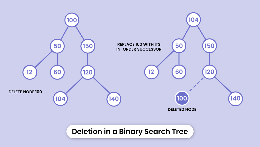
In the picture, deleting 100 (which has two children) copies in 104, the smallest node in 100's right subtree, and then removes the original 104. The same case in Python:
def delete(root, value):
    if root is None:
        return None
    if value < root.value:
        root.left = delete(root.left, value)
    elif value > root.value:
        root.right = delete(root.right, value)
    else:
        if root.left is None:            # leaf, or only a right child
            return root.right
        if root.right is None:           # only a left child
            return root.left
        successor = root.right           # two children: find the in-order successor,
        while successor.left is not None:    # the smallest key in the right subtree
            successor = successor.left
        root.value = successor.value
        root.right = delete(root.right, successor.value)
    return root

bst = delete(bst, 100)                   # the case from the picture
print(inorder(bst, []), bst.value)       # [12, 50, 60, 104, 120, 140, 150] 104
Time complexity of tree operations
Search, insertion and deletion in a binary search tree follow one path from the root, so they cost O(h), where h is the height. The height depends on the shape of the tree:
| Tree | Search, insert, delete | Why |
|---|---|---|
| Balanced BST (for example AVL) | O(log n) | The height stays about log n, because every level roughly halves the nodes left to search |
| Skewed BST (a degenerate tree) | O(n) | Every node has one child, so the tree behaves like a linked list |
| Any traversal | O(n) | Each node is visited once |
Insert 1, 2, 3, 4, 5 in that order into an empty binary search tree and you get a skewed tree of height 4. Insert 2, 1, 3 and you get a balanced tree of height 1. Self-balancing trees such as AVL and red-black trees avoid the bad case (Java's TreeMap is a red-black tree).
Applications of Tree Data Structure
Trees store data that is naturally hierarchical, or data that has to stay sorted. This is a short tour; the guide to the applications of the tree data structure covers more.
| Where | Which tree | What it does |
|---|---|---|
| File systems | A tree of folders | Drives contain folders, folders contain subfolders and files: a natural hierarchy |
| Ordered maps and sets | Self-balancing binary search trees | Search, insert and delete in O(log n) with the keys kept in sorted order (Java's TreeMap is one) |
| Database indexes and file systems | B-trees | Wikipedia calls the B-tree the standard index structure in almost all relational databases, and file systems such as NTFS and ext4 use it too |
| Autocomplete and spell checking | Tries (prefix trees) | Words that share a prefix share a path, so finding everything that starts with a prefix is fast. Search-as-you-type is the classic use |
| Routers | Compressed tries | Store IP address prefixes so a router can look up the next hop by prefix |
| Compilers | Syntax trees | Programmers also use syntax trees in compilers to represent and check the structure of the programs they write |
When to use a tree (and when not to)
| You need | Pick | Why |
|---|---|---|
| Data that is naturally nested: folders, an org chart, comments and replies | A tree | The structure of the data is a tree |
| Keys in sorted order, range queries or the next larger key | A balanced binary search tree | O(log n) per operation, and an inorder walk gives the keys sorted |
| Look-ups by key where order does not matter | A hash map | O(1) on average, against O(log n) for a balanced tree |
| Search in a fixed, already sorted list | A sorted array and binary search | Simpler and uses less memory, but inserting is slow |
| An index too big for memory, stored on disk | A B-tree | Each node holds many keys, so a lookup reads few disk blocks |
Classic tree interview problems
Almost every tree question comes down to a traversal and a base case (usually the empty tree). Five classics:
| Problem | Idea |
|---|---|
| Maximum Depth of Binary Tree | The depth is 1 plus the larger of the left and right depths. An empty tree has depth 0. |
| Invert Binary Tree | Swap the left and right child of every node, recursively. |
| Validate Binary Search Tree | Pass down the allowed range (low, high) for each node, or check that the inorder traversal is strictly increasing. |
| Binary Tree Level Order Traversal | Run BFS with a queue and process one whole level at a time. |
| Lowest Common Ancestor of a BST | Start at the root. If both values are smaller, go left. If both are larger, go right. Otherwise the current node is the answer. |
Final Thoughts
We hope you got the gist of the tree data structure. And it’s important to understand all data structures and algorithms if you want to become a top-notch programmer. DSA helps in building logic and problem-solving skills that are quite useful in real life too. (Here are 5 important reasons to learn DSA)
Case in point, if you have to list all the employees in an organization with their respective positions in mind, you can do so easily using the principle of a tree data structure. It’ll define the hierarchy of employees and make it easy for others to reach out to specific individuals.
Just look around and you’ll find innumerable examples of various data structures and algorithms in play.
If you want to clarify the concept of data structures and algorithms from scratch, refer to this article.
Happy Coding!
FAQs
What does a tree structure in programming mean?
A tree is a hierarchical data structure: one root node at the top, and every other node has exactly one parent and zero or more children. Nodes are joined by edges, there are no cycles, and a tree with n nodes has n - 1 edges.
What are the types of trees in data structure?
The common types are the general tree, the binary tree (with full, perfect, complete, degenerate and balanced forms), the binary search tree, the AVL tree and the B-tree. Red-black trees and tries are two more you meet in practice.
What is the difference between a binary tree and a binary search tree?
A binary tree only limits each node to two children. A binary search tree adds an ordering rule: keys in a node's left subtree are smaller and keys in its right subtree are larger. That lets it be searched in O(h) time, and an inorder walk returns sorted keys.
What is the difference between the height and the depth of a node?
Depth counts the edges from the root down to the node, so the root has depth 0. Height counts the edges on the longest path from the node down to a leaf, so a leaf has height 0.
What is the difference between a tree and a graph?
A tree is a connected graph with no cycles, so any two nodes are joined by exactly one path, and it has a root. A general graph can have cycles, can be disconnected and can be directed. Every tree is a graph, but not every graph is a tree.
What is the time complexity of searching a binary search tree?
It is O(h), where h is the height. In a balanced tree, such as an AVL tree, that is O(log n). In a skewed tree, where every node has one child, it degrades to O(n), like a linked list.