Applications of Graph Data Structure

Graph data structures and algorithm concepts can be easily understood, given you learn them correctly.

Have you ever wondered how you get mutual friends' suggestions on social media platforms? Or even the ‘people who bought this also bought this’ suggestions on E-commerce platforms? Graph data structure is the answer.

What is graph data structure?

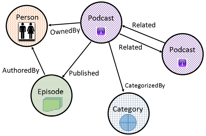
A graph is a non-linear data structure, a collection of nodes connected to each other via edges. Each node contains a data field and the edges act as an interaction between two data fields.

Simplifying it further, we get-

• A collection of nodes also known as vertices
• A collection of edges E connecting the vertices, (represented as ordered pair of vertices- 1, 2)

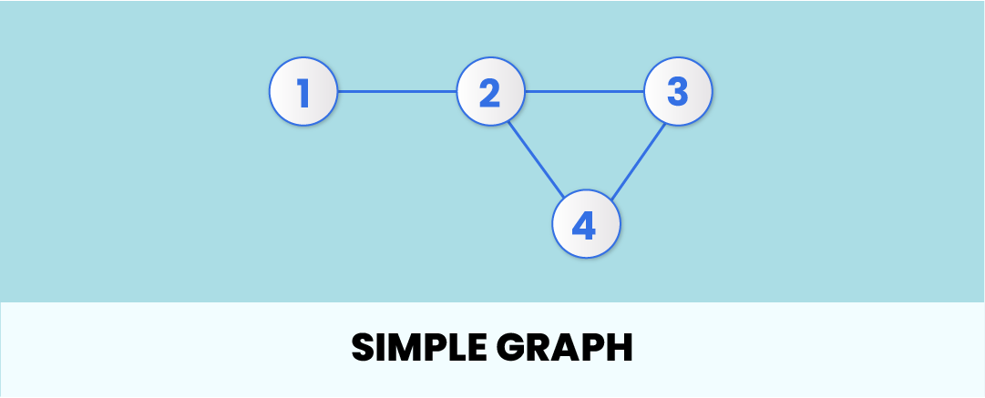
It is a versatile data structure that enables us to model and depict numerous real-world phenomena. Before we proceed, let's take a moment to visualize a graph.

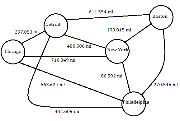
Imagine a network of cities connected by roads. Here, each city can be considered a vertex or node, and the roads that connect them are the edges of the graph.

If you look closely, the entire universe could be a graph in and of itself. We can imagine the cosmos beginning as a set of abstract relationships between abstract elements. Some researchers do have explanations for this hypothesis as well. (I’m attaching one of the studies here in case you want to delve deeper)

Here are some of the key features and properties of graphs:

1. Nodes (Vertices):

• Nodes are the fundamental elements of a graph.
• Each node typically represents an entity, object, or data point.
• Nodes can be labeled to provide additional information about what they represent.

2.  Edges (Arcs/Links):

• Edges are the connections between nodes.
• They represent relationships, interactions, or connections between the entities represented by the nodes.
• Edges can be directed (point from one node to another) or undirected (bi-directional).

3.  Types of Graphs:

• Directed Graph (Digraph): Edges have a direction, indicating a one-way relationship.
• Undirected Graph: Edges have no direction, representing mutual relationships.
• Weighted Graph: Each edge has a weight or cost associated with it, often used in optimization problems.
• Cyclic Graph: Contains at least one cycle (a path that starts and ends at the same node).
• Acyclic Graph: Does not contain any cycles.
• Connected Graph: There is a path between every pair of nodes.
• Disconnected Graph: Contains one or more isolated subgraphs.

4.  Degree of a Node:

• The degree of a node is the number of edges connected to it.
• In a directed graph, there are both in-degrees (incoming edges) and out-degrees (outgoing edges) for each node.

5.  Adjacency:

• Two nodes are adjacent if there is an edge connecting them.
• The adjacency matrix or list is used to represent which nodes are adjacent in a graph.

6.  Path:

• A path is a sequence of nodes where each adjacent pair is connected by an edge.
• The length of a path is the number of edges it contains.

7.  Connected Components:

• In an undirected graph, a connected component is a subgraph in which there is a path between any two nodes.
• A graph may have multiple connected components.

8.  Cycle:

• A cycle is a path that starts and ends at the same node, forming a closed loop.
• Acyclic graphs have no cycles.

9.  Graph Traversal:

• Graph traversal algorithms like depth-first search (DFS) and breadth-first search (BFS) are used to explore or search through the nodes and edges of a graph.

10. Graph Representation:

• Graphs can be represented using various data structures, including adjacency matrices, adjacency lists, and edge lists.

11. Applications:

• Graphs are used in various applications, including social networks, transportation networks, computer networks, recommendation systems, and more.

12. Planar Graphs:

• A graph is planar if it can be drawn on a plane without any edges crossing except at their endpoints.

13. Eulerian and Hamiltonian Paths:

• An Eulerian path is a path that visits each edge of a graph exactly once.
• A Hamiltonian path is a path that visits each node of a graph exactly once.

These are some of the fundamental features and properties of graphs. Depending on their specific characteristics and applications, graphs can exhibit many more complex properties and behaviors.

Now we’ve already covered graphs in detail in our previous article. Here, we’ll focus on the real-world applications of graphs that we can actually see and experience, scenarios where the principles of graph data structures are applicable:

• Social Networks
• Google Maps
• Web Crawlers
• Recommendation Engines
• Program Dependencies

Let’s look at each of them in detail:

Social Networks

Have you ever wondered how these platforms are so adept at suggesting connections or "friends"? In these networks, each user is represented as a node or vertex, and their connections are the edges of the graph.

Utilizing graph algorithms like Depth First Search(DFS) or Breadth-First Search (BFS), these platforms can identify the connection (or sometimes, the degrees of separation) between two users.

Depth-First Search (DFS)

Depth-First Search (DFS) is an algorithm used to traverse or search a graph in a depthward motion. It uses a stack data structure to remember to get the next vertex to start a search when a dead-end occurs in any iteration.

Here's a high-level view of how it works:

• Start from the root or any arbitrary node (this typically becomes the 'source' node).
• Explore the adjacent nodes of the current node.
• Go deep into the graph by visiting the next adjacent node.
• When you visit a node that has no adjacent nodes that you haven't visited yet, you go back to the previous node and visit another node from its adjacent nodes.
• Repeat the steps until all nodes are visited.

The DFS algorithm's pseudo-code can be implemented in the following way:

DFS(Graph, start_vertex):
    create a stack S and push start_vertex into it
    create a set (or list) V to track visited vertices
    while S is not empty:
        current_vertex = S.pop()
        if current_vertex is not in V:
            add current_vertex to V
            for every neighbor of current_vertex:
                push neighbor into S

Breadth-First Search (BFS)

It's another algorithm used to traverse or search a graph in a breadthward motion. It uses a queue data structure to remember to get the next vertex to start the search when a dead-end is met.

Here's a high-level view of how it works:

• Start from the root or any arbitrary node (this typically becomes the 'source' node).
• Visit all the unvisited neighbors of the current node, then for each of those neighbor nodes, visit their unvisited neighbors.
• Continue this process level by level until all nodes are visited.

The BFS algorithm's pseudo-code can be implemented in the following way:

BFS(Graph, start_vertex):
    create a queue Q and enqueue start_vertex into it
    create a set (or list) V to track visited vertices
    while Q is not empty:
        current_vertex = Q.dequeue()
        if current_vertex is not in V:
            add current_vertex to V
            for every neighbor of current_vertex:
                enqueue neighbor into Q

The platforms use these algorithms to find the shortest path between nodes, or the degrees of separation between users. For instance, if user A is a friend of user B, and user B is a friend of user C, then the platform can suggest user C as a potential friend to user A, as they are two degrees separated.

These algorithms are also used in features like feed generation, community detection, finding people you may know, and even for pushing appropriate ads to users.

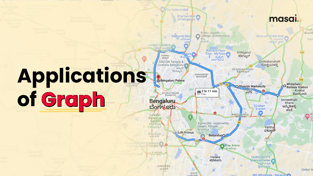
Google Maps

Graphs have transformed the way we navigate our world, quite literally. Whether you're mapping out a road trip or finding the quickest route to your favorite restaurant, chances are you're using Google Maps. But how does it calculate the shortest route between your current location and destination?

In the case of Google Maps, locations, such as cities or specific addresses, are represented as vertices (or nodes), and the roads or paths between them are represented as edges. Each edge has an associated weight, which could represent various metrics like distance, time, or traffic conditions between two vertices.

Two of the most commonly used algorithms in route-finding applications are Dijkstra's Algorithm and the A* (A-Star) Search Algorithm.

Dijkstra's Algorithm

Dijkstra’s Algorithm works by visiting vertices in the graph starting from the object's start condition, and it extends the current path as long as it continues to find shorter paths.

Here's the pseudocode of Dijkstra's Algorithm:

This algorithm will return the shortest distance from the source to all other vertices, and a map of previous vertices, which can be used to reconstruct the shortest path from the source to any other vertex.

Dijkstra(Graph, source):

  create vertex set Q

  for each vertex v in Graph:            
    distance[v] ← INFINITY                 
    previous[v] ← UNDEFINED                
    add v to Q                     
  distance[source] ← 0               
 
  while Q is not empty:
    u ← vertex in Q with min distance[u]  
    remove u from Q 
       
    for each neighbor v of u:           
      alt ← distance[u] + length(u, v)
      if alt < distance[v]:              
        distance[v] ← alt
        previous[v] ← u

  return distance[], previous[]

A* Search Algorithm

It is a more sophisticated method that also takes into account the 'heuristic' - an educated guess of which node to explore next based on additional information. This heuristic is often the straight-line distance from the current node to the goal.

The A* Search Algorithm prioritizes paths that are likely to be more efficient. It does this by maintaining a priority queue of paths based on the cost function f(n) = g(n) + h(n), where g(n) is the cost from the start node to node n, and h(n) is the heuristic estimate of the cost from node n to the goal.

Here is a high-level view of A* Search Algorithm:

A*(start, goal):
  create a priority queue Q of paths
  add start to Q with cost 0
  while Q is not empty:
    current = node in Q with the lowest f(n)
    if current is goal:
      return current
    for each neighbor of current:
      if neighbor has not been visited:
        add neighbor to Q with cost g(neighbor) + h(neighbor)

It is efficient and finds the shortest path if such a path exists. The addition of a heuristic allows it to make intelligent decisions about which nodes to explore, which can drastically reduce the time spent searching, especially in large graphs.

When you search for the shortest path between your current location and a destination, these algorithms run behind the scenes, determining the best route based on factors like distance, time, and current traffic conditions. As a result, we can reach our destinations following the most optimal paths.

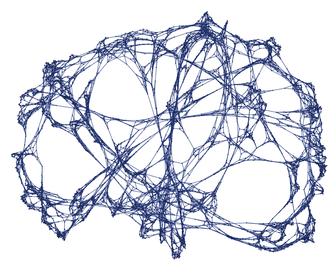
Web Crawlers

At a fundamental level, the World Wide Web is a massive, interconnected graph. Each webpage or URL can be viewed as a node, and the hyperlinks that connect these pages act as edges, creating a colossal graph structure.

For example, Google employs web crawlers (also known as spiders or bots) to traverse the web, indexing web pages for its search engine. The web crawler starts with a list of URLs to visit, known as the seed. As it visits these URLs, it identifies all the hyperlinks on the page, adding them to the list of URLs to visit. This method of traversal, known as a graph traversal algorithm, is used by Google to index billions of web pages on the internet.

The main goal of a web crawler is to index the web pages it visits, creating a catalog that can be used by search engines like Google to deliver relevant search results.

The basic algorithm that a web crawler might use can be represented in pseudocode as follows:

function WebCrawler(seedURL):
  create a Queue and enqueue seedURL
  while Queue is not empty:
    URL = Queue.dequeue()
    if URL is not yet visited:
      mark URL as visited
      download and index the content of URL
      for each link in the webpage corresponding to URL:
        Queue.enqueue(link)

This algorithm resembles the Breadth-First Search (BFS) algorithm, as it visits all the directly connected nodes (web pages linked from the current page) before moving on to the next level of nodes.

Web crawlers can also use other graph traversal algorithms depending on the specific requirement. For example, a BFS-based crawler would be more suitable if we want to first index pages that are fewer clicks away from the seed page. On the other hand, a DFS-based crawler might be more efficient in terms of memory usage.

Recommendation Engines

If you've used platforms like Amazon, Netflix, and Spotify, you've likely noticed how accurately they suggest products or movies based on your browsing history. This is no accident, and once again, graphs are the hero of this story.

Recommendation engines use graph algorithms to connect similar items and recommend them to users. These engines operate by creating a graph where the nodes represent users and items, and the edges represent interactions between users and items (like a user rating a movie). The weight of the edge often represents the strength of the interaction (e.g., the rating a user gave to a movie).

They then use algorithms to analyze these graphs and make recommendations. The principle of "people who bought this also bought..." is a perfect illustration of the usage of graphs in recommendation engines.

A key feature of graph-based recommendation systems is their ability to model more complex relationships. For example, a node in the graph could represent not just a user or an item, but also an attribute of an item, such as its category or brand. Edges can then represent not just interactions between users and items, but also relationships between items based on their attributes.

Graph-based algorithms such as PageRank can then be used to rank items in the graph based on their relevance to a given user. The personalized PageRank algorithm, for example, starts with a random walk on the graph from a given user node and ranks items based on their visit frequency during the walk.

This way, graph-based recommendation systems can leverage both the interaction data and the attribute data to provide more accurate and personalized recommendations.

Program Dependencies

In any non-trivial software development project, it's normal to have a web of dependencies that need to be managed. These dependencies could be between different libraries, modules, classes, or even functions within the code.

To help manage these dependencies, developers often use graphs, where each node represents a unit of code (like a library or module), and each edge represents a dependency between two units.

These graphs are usually directed, meaning that the edges have a direction that indicates which way the dependency goes. For instance, if library A depends on library B, there would be an edge from A to B.

To prevent circular dependencies, these graphs are typically acyclic, meaning they don't contain any cycles. These types of graphs are known as Directed Acyclic Graphs (DAGs).

One of the most common operations performed on DAGs is topological sorting. This algorithm is used to find a linear ordering of the nodes that respects the partial order defined by the edges. In other words, if there is a directed edge from node A to node B, then A appears before B in the ordering.

There are several algorithms to perform topological sorting, including Kahn's algorithm and the depth-first search (DFS) based algorithm.

Don't Leave Just Yet

So, these were the 5 important applications of graphs in detail. But there are many more. And we can’t let you go without mentioning a few more, just can’t keep them to ourselves.

Computer vision- Graphs act as a vital tool to represent and interpret image and video data with object tracking and edge detection.

Natural language processing- In this context, they provide a structured way to analyze and represent textual data, such as in syntactic and semantic dependency graphs.

Bioinformatics- Biological data such as genetic networks and protein-protein interactions are modeled and analyzed using graphs.

Artificial Intelligence- Graphs help model complex relationships in data, helping develop sophisticated predictive models and enabling machines to understand and generate human-like responses.

Understanding and applying graph data structures and algorithms is an essential skill set for anyone looking to advance in the fields of computer science, data analysis, and beyond.

To know more about graph data structures, check out this article.

To understand the concept of data structures and algorithms from scratch, click here.

If you're ready to take your coding and DSA skills to the next level and turn your career aspirations into reality, check out our pay-after-placement courses and start your journey today.